


Measuring the Coating Window: Simplify the Concept with Mapping
- Published: June 24, 2024
By Ted Lightfoot, PhD - Casting, coating, drying and laminating film consultant
 Coating windows are the most useful way to understand what is going on at the coating head. A coating window is a two dimensional map of which combinations of settings give uniform coatings and which give defects. Most people are familiar with the concept, but many struggle with how to apply it.
Randomly adjusting the settings on any piece of manufacturing equipment might or might not produce good product. This is certainly true of the coating process. The control settings vary from one coating method to the next. But line speed, viscosity and surface tension are always important. So, the operability region is really a four or more dimensional object.
How do we make sense of an operating window in four or more dimensions? Break it down into a series of two dimensional maps that can be measured efficiently and understood easily. The first map to draw is a window often called an "operability diagram." This is best explained by a (made up) example:
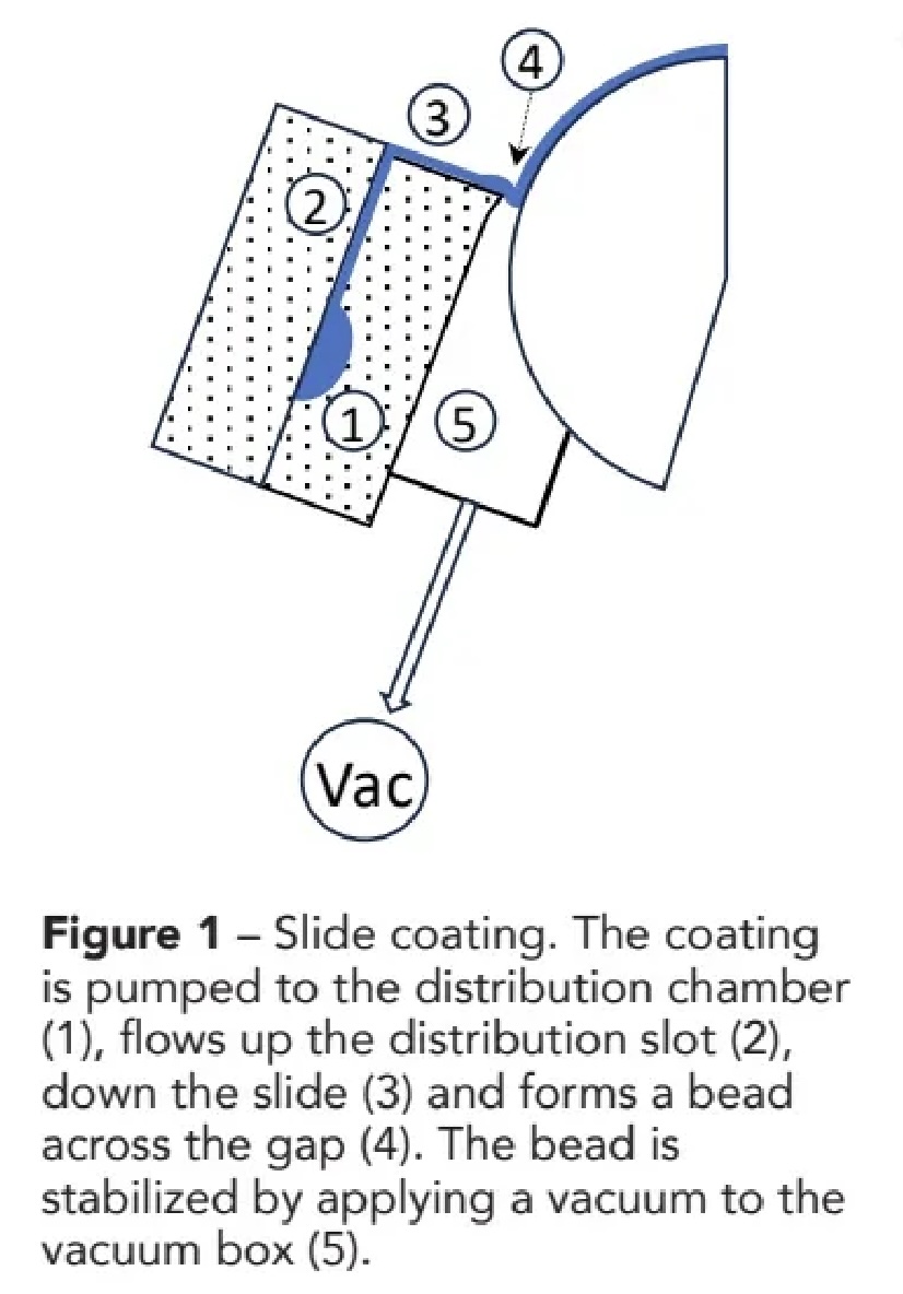
We will work through the mapping process for the slide coater sketched in figure 1 because the most detailed window ever published (figure 2b) is for slide coating.
Step 1: Planning
Start by listing and ranking factors in terms of how quickly they can be manipulated. The settings for slide coating are listed in table 1 along with an order of magnitude estimate of how quickly they can be changed. For example, depending on the magnitude of the change and the acceleration of the line, speed changes usually take between five and 50 seconds (0.5-5.0 x 101 seconds).
Using the ranking in table 1, we will map the effects of vacuum at different line speeds to produce a two dimensional map at a fixed gap, surface tension and viscosity. We will repeat this at various gaps before changing the formulation and repeating the whole process. One convenient feature of slide coating is that by keeping pump speed proportional to line speed, the coating weight is kept constant.
Step 2: Start Inside the Coating Window
How do we do that without knowing the window? Trial and error. But most coating windows are wider at low speed than at high speed - and we waste less material at low speed. So, we start slow (25 fpm) with a moderate vacuum (1"WC). Unfortunately, slide coating often has a minimum speed, so we get a barring defect. But this is well known (and not the case with most other methods). So, we jump up to 50 fpm and the detect goes away.
Step 3: Measure the Upper Limit
Our window is defined by the range of a vacuum that doesn't produce gross defects. There are two approaches to measuring the limits: We can run a set of defined vacuum levels or adjust the vacuum continuously. Measuring at discrete points does not pinpoint the boundary between operable and inoperable states and we want to track the boundaries.
So, in most cases, we adjust the vacuum continuously noting where a defect appears. In our example, at 50 fpm, we turn the vacuum up until ribbing appears at 1.5 "WC. But streaks and ribbing sometimes appear gradually. In these cases, we want to run at fixed points to quantify how quickly/slowly the defect appears/disappears. If we start by adjusting continuously and notice a gradual transition, we can always pivot to running patches at different vacuum levels for optical analysis.
Step 4: Measure the Lower Limit
Now, we go the other way and drop the vacuum until we find a different defect. In our example, when we get down to 0.05 "WC, the bead breaks at the edges. We then bring the vacuum back up to get back into the coating window. If we are lucky, the edge reestablishes itself (at 0.1" WC). If we are unlucky, it may take operator intervention to reestablish a stable edge. But, even if we are lucky, we have encountered another complication: We might get good coating under certain conditions and we might not — depending on how we got there.
Step 5: Change Line Speed and Repeat
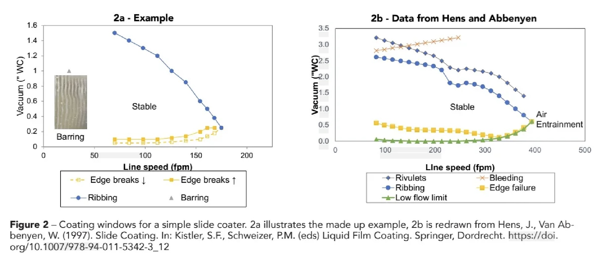
We repeat this process at different line speeds to generate the coating window shown in figure 2a. Of course, we could be more thorough and produce a comprehensive diagram such as shown (for a real process) in figure 2b.
Comparing figure 2a and 2b, we see that figure 2b shows the boundary as sharp lines — no defects seem to appear gradually and there is no hysteresis at low vacuum as shown in figure 2a. How did they get these sharp lines? First, their broken edges may not have healed themselves. Some people choose the narrowest limit (as long as we are above that, we should never get the defect). Other people choose the widest limit (this is often the best choice for statistical process control). The most common approach is to let the operator use their judgement (and possibly a piece of shim stock) to determine a limit. If a pattern occurs gradually, we have to determine what level of variation our customers will accept. Always consider the context before defining ambiguous limits.
Figure 2b shows more defects than our example and has high resolution. This may be appropriate for documentation at product commercialization. But the most significant difference between figure 1a and 2b is the range of line speeds. Is our speed limited by coating thickness, gap, viscosity, or surfactant level? We are often best to run multiple low resolution windows at different conditions. There are other two dimensional maps that help us optimize our product and process. We will talk about some of these in future articles.
About the Author
E.J. (Ted) Lightfoot has worked in coating, drying and laminating for almost 40 years. He has experience in R&D, plant support, as a Six Sigma Black Belt for Growth, helping customers develop products and processes as well as numerous defect reduction projects. Ted works as a consultant, writer and teaches short courses. He can be reached at This email address is being protected from spambots. You need JavaScript enabled to view it..